With just a handful of examples, a fine-tuned open source embedding model can provide greater accuracy at a lower price than proprietary models like OpenAI’s text-embedding-3-small. In this article, we’ll explain how to create one with Modal. First, we’ll cover the basics of fine-tuning. Then, we’ll talk about an experiment we ran to determine how much fine-tuning data we needed for a simple question-answering use case.

The why of fine-tuning

Open models get you started

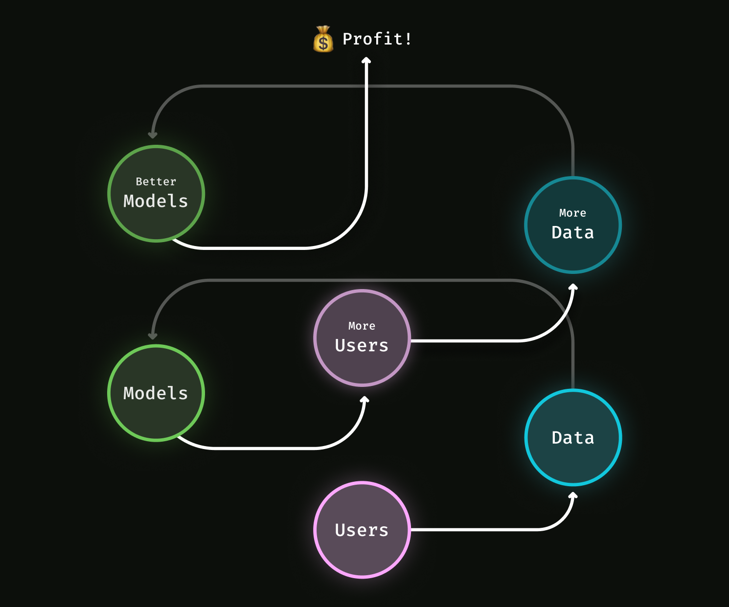
Custom models matter. That’s how Netflix keeps suggesting better movies and how Spotify manages to find a new anthem for your daylist. By tracking when you finish the movie you chose or whether you skipped a song, these companies accumulate data. They use that data to improve their internal embedding models and recommendation systems, which lead to better suggestions and a better experience for you. That can even lead to more engagement from more users, leading to more data, leading to better models, in a virtuous cycle known as the data flywheel.

Large, ML-forward organizations like Netflix and Spotify have taken advantage of data flywheels to create their own models from scratch, and now they have lots of data. But when you’re just starting out on a new company or project, you don’t always have the data you need. Bootstrapping a data flywheel in the 2010s required substantial creativity or resource investment.

But the advent in the 2020s of highly capable, generic pre-trained models with permissive licenses has dramatically simplified that bootstrap step. You can start with one of these models, trained to recognize patterns in a large, diverse dataset, and expect them to perform reasonably well on your task.

In a previous blog post, we demonstrated this by deploying an off-the-shelf model on hundreds of GPUs using Modal’s autoscaling infrastructure, embedding the entirety of English Wikipedia in under 15 minutes.

Fine-tuning kicks off the data flywheel

The availability of both these models and the infrastructure to run them easily is great news for organizations which are just starting out and don’t have any user data yet. But it’s critical to move as fast as possible to a custom model that delivers better performance than the off-the-shelf model. Luckily, data accumulates quickly: just a few dozen users interacting with a service only 3-4 times per day can create hundreds of datapoints in a matter of days.

And that’s all the data we needed to train a model that could beat OpenAI’s text-embedding-3-small at identifying textual similarity on a sample dataset.

The same scalable, serverless infrastructure on Modal that we used to create embeddings with the off-the-shelf model can also be used to customize it, a process called fine-tuning. The end result is an ML application with superior performance at a significantly reduced operational expense: the first step to starting your own data flywheel.

The how of fine-tuning: datasets, models, and infrastructure

When fine-tuning a model, there are a number of design decisions that must be made. We review a few of them here.

Finding or creating a dataset

Though much of the discussion and research in machine learning is around models, any ML engineer worth their salt will tell you that the dataset is the most critical component.

Embedding models are generally trained on datasets made out of pairs of items, where some pairs are marked as “similar” (like sentences from the same paragraph) and some are marked as “different” (like two sentences chosen at random). The same principle could be applied to longer texts than sentences — paragraphs, pages, documents — or it could be applied to things other than text — images, songs, user clickstreams — or it could be applied to multiple modalities at once — images and their captions, songs and their lyrics, user clickstreams and purchased products.

We’ll be using the Quora dataset, which contains pairs of questions from posts on Quora, where some pairs are questions that have been marked as duplicates.

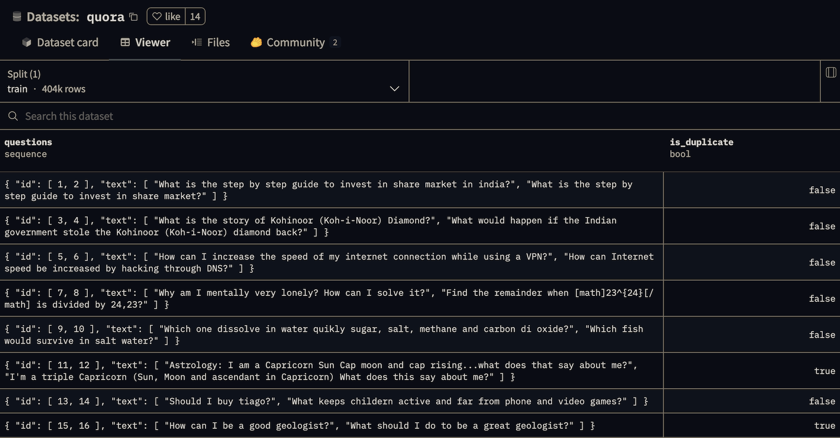
You can review the dataset in an interactive viewer here. Some of the question pairs, like “Can I hack my Charter Motorolla DCX3400?” and “How do I hack Motorola DCX3400 for free internet?”, are quite similar, but are not duplicates, aka they are “hard negatives”.

Together, that makes the model we’re training here potentially useful for retrieval-augmented generation (RAG) chatbots. In embedding-based RAG for chatbots, a large corpus of text must be searched for a small number of passages that “match” a query from a user, aka likely contain the answer. This dataset will train the model to be sensitive to very small differences in the topic of a question. Near duplicates can also be removed before retrieval or before training other models, a technique known as “semantic deduplication”.

Choosing a base model

We’ll primarily be focusing here on permissively licensed, weights-available models. These models have weights that you can download and modify the same way you download and modify open source code. For that reason, we refer to them here as “open source” models, even though there is no Open Source Initiative-sanctioned definition of “open source” that applies to models. Models are commonly released via Hugging Face’s git LFS-based model repository hub, and that’s where we’ll get our models.

Alternatively, we could have used an API to fine-tune a proprietary model, as is offered by some embedding API services. In addition to concerns about cost, we find that fine-tuning a model is sufficiently complex and use-case-specific that controlling the training process is necessary.

How do you choose between available models? Each model is trained differently and with a specific use-case in mind. Most critically, a model is trained on a specific modality or modalities (text, images, audio, video, et cetera) and a specific set of data. Once you have narrowed down to models that handle the modalities in your use case, compare their performance on public benchmarks, like MTEB. In addition to task performance, review the model’s performance in terms of resource requirements and throughput/latency, again via public benchmarking data (hardware providers like Lambda Labs are a good resource here).

For example, the embedding dimension, or the number of entries in the output embeddings of the model, is an important consideration. Larger vectors can store more information, leading to better task performance, but can result in significantly higher costs (costs scaling more like RAM than like disk) as we embed more data over time. When fine-tuning, we can adjust this dimension.

Acquiring training infrastructure

Fine-tuning a model requires significant compute resources. Even models that can later be run satisfactorily on CPUs, even client or edge CPUs, are frequently trained on GPUs, which can achieve high throughput on easily parallelizable workloads like training.

For a typical fine-tuning job, we need one to eight server-grade GPUs. More than eight GPUs generally requires distributing training over multiple nodes, due to connectivity constraints, which significantly increases both hardware cost and engineering complexity.

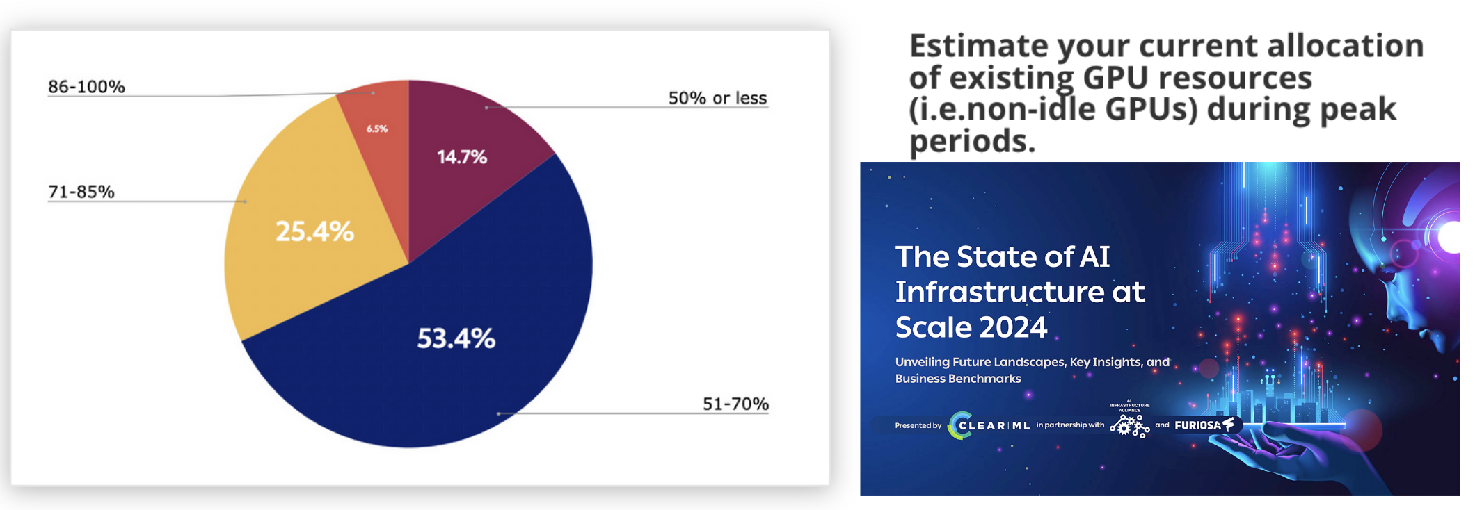
But server-grade GPUs are scarce these days, meaning they are expensive to purchase or rent and cloud providers frequently require reservations of a minimum size and duration. But fine-tuning jobs are less like production workflows (always on, reasonably predictable traffic) and more like development workflows (intermittent, unpredictable). Combined, these phenomena have lead to massive over-allocation and over-spending, with organizations reporting peak utilizations of about 60% on average, according to this survey from ClearML and the AI Infrastructure Alliance — and even less off-peak.

Modal solves this problem: it provides autoscaling infrastructure, including GPUs, so you only pay for what you use (aka it is “serverless”). Modal also offers a Pythonic, infrastructure-from-code interface, empowering data scientists and ML researchers to own and control their infrastructure.

With these resources in hand, we need to determine how to scope our model training process. The more time and money we spend on training, iterating on hyperparameters and data tweaks, the better our task performance will become, but with diminishing returns. In general, we recommend either training to satisfaction on some metric (e.g. at least 90% accuracy) or selecting a number of metrics to satisfy and one metric to maximize (e.g. highest accuracy we can get with recall ≥ 50%), then setting a hard limit on resources and time.

Running a grid search over fine-tuning hyperparameters

Determining how to train an entirely new model architecture or on an entirely new task is a research project, and should be scoped accordingly. But fine-tuning is simpler — we can use pre-existing training recipes, like the ones used to train the model (if it has been open-sourced). But there is still room for experimentation, including on many of the considerations listed above.

We selected as experimental parameters the three we considered most important: which pre-trained model should we train, on how much data, and with how many output dimensions? Because these experimental parameters determine the values of the parameters (the weights and biases) in the model, they are known as hyperparameters.

The simplest way to explore hyperparameters is to define a set of possible values for each hyperparameter and then check all combinations — a grid search. This is a brute-force approach, but, as we’ll see below, it is effective and easy to parallelize.

We added two additional models to the original bge-base-en-v1.5 model we used in the Wikipedia embedding example and we tried two different embedding dimensions. For each of these configurations, we tested a different dataset size, ranging from one hundred to over one hundred thousand samples:

MODELS = [
    "BAAI/bge-base-en-v1.5",
    "sentence-transformers/all-mpnet-base-v2",
    "jinaai/jina-embeddings-v2-small-en",
]
DATASET_SIZE = [
    100, 200, 400, 800, 1600, 3200,
    6400, 12800, 25600, 51200, 102400,
]
DENSE_OUT_FEATURES = [256, 512]

All other hyperparameters were held fixed.

Next, we generated all possible combinations of model, dataset_size and dense_out_features using the product function provided by the standard library module itertools, which creates an iterator that returns every possible combination of elements from each of the input lists (aka the Cartesian product). We then use these combinations to generate configuration objects for our model fine-tuning process:

def generate_configs():
    for model, sample_size, dense_out_features in product(
        MODELS, DATASET_SIZE, DENSE_OUT_FEATURES
    ):
        yield grid_search_config(model, sample_size, dense_out_features)

Whatever our fine-tuning process is, it takes configs and produces some dictionary of results. We wrap it in a function that we decorate with @app.function() to make it runnable on Modal’s autoscaling infrastructure, as in the pseudo-code below.

@app.function(gpu="A10G")  # configure autoscaling and other infra parameters here
def objective(config) -> dict:
    model = Model.from_config(config)
    model.setup()
    results = model.train()
    return results

From there, scaling is as simple as calling objective.map to run experiments in parallel. We wrap this in a function that we decorate with @app.local_entrypoint() so that we can launch experiments from the command line with modal run.

@app.local_entrypoint():
def run():
    results = []
    for experiment_result in objective.map(generate_configs()):
        results.append(experiment_result)

    df = pd.DataFrame(results).sort_values("metric_accuracy", ascending=False)
    df.to_csv("trial_results.csv", index=False)

Our training process fits on a single GPU, and each experiment runs in parallel, so we can scale it all the way up to the maximum number of simultaneous GPU workers allowed in Modal — in the thousands, at time of writing. For large training jobs, this can mean the difference between getting results next week or after lunch.

Beating proprietary models with a few hundred examples

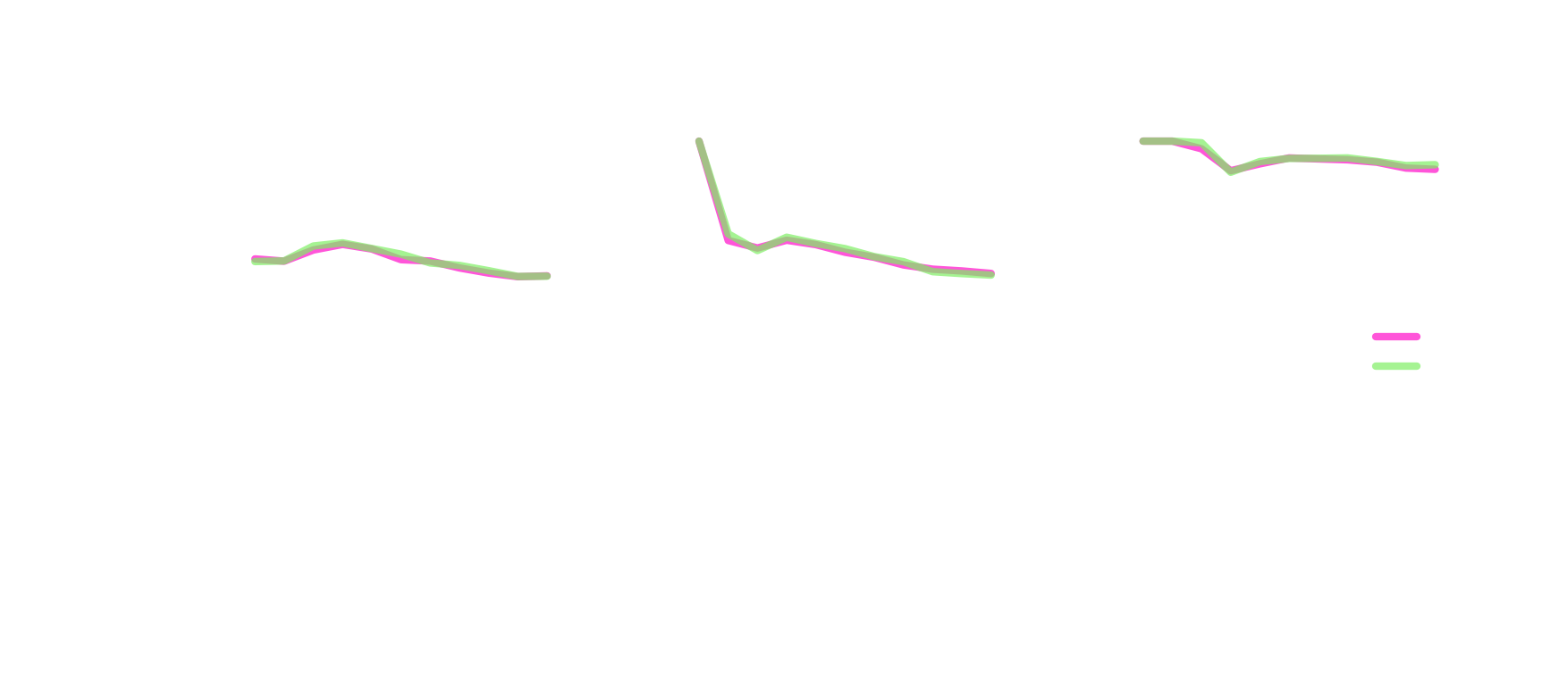
The figure below summarizes the results of our experiment, showing the error rate (fraction of predictions that are incorrect) of the models we trained on the Quora dataset as a function of the number of dataset examples used during fine-tuning, with one plot for each of the three models. The performance of the OpenAI text-embedding-3-small model is shown for comparison. For completeness, we show the two different embedding dimension sizes we tested, though we didn’t observe a difference in performance between them for any setting of the other hyperparameters.

We see a few patterns commonly observed in fine-tuning in these three cases:

• For the jina-embeddings-v2-small-en model, the error rate is higher than the baseline and never goes down. As always, it’s plausible that different settings of the other hyperparameters we didn’t tune might lead to improved performance from this model. These are the kind of results you don’t want to get from a hyperparameter search, because it’s not clear what to do next.
• For the all-mpnet-base-v2 model, the error rate is lower than the baseline after just 100 examples, but we don’t observe much improvement, even out to three orders of magnitude more examples.
• For the bge-base-en-v1.5 model, the error rate starts out higher than the baseline model, but rapidly improves with more data, convincingly beating the baseline by 200 examples and still improving at 100,000 examples.

Reviewing these results, we’d move forward with the fine-tuned bge-base-en-v1.5 model, especially if we expected to be able to collect more data via a data flywheel in the future. We’d most likely select the 256-dimensional embeddings, as they are cheaper to produce and store than the 512-dimensional embeddings, and we didn’t observe an accuracy benefit from using the larger embeddings.

You might object that the improvements over the baseline are small in absolute terms — an error rate of 17% versus an error rate of 13%. But relatively, that is a large difference: a full quarter of the mistakes that the baseline model makes are avoided by the fine-tuned model. This phenomenon gets stronger as the error rate decreases: a system with 99% reliability can be used in situations where one with 95% reliability is inadmissible, even though the magnitude of the difference seems small.

Next steps

In this article, we’ve shown how to fine-tune an open source embedding model to beat a proprietary model on a simple question-answering task. We’ve also discussed the considerations that go into fine-tuning a model and how to run a grid search over hyperparameters using Modal. We’ve shown that even with just a few hundred examples, we can achieve better performance than proprietary models.

Moving forward, the next step in fine-tuning would be to operationalize this process, so that we can collect more data and iterate on the model. With full automation, we could even turn the model into a continuously-improving system, powered by the additional data we collect.

Far more than models, these pipelines and processes for converting data into useful features for users are the output of machine learning teams. With open source models and serverless infrastructure, building them is easier than ever.